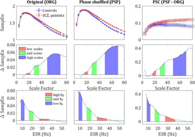
Figure 1a depicts the grand average SampEn across subjects and sensors as a function of the scale factor. Consistent with previous studies, the SampEn was significantly higher in SCZ patients compared to controls16,42,43. A higher entropy was observed in 216 of 273 channels. The grand average of a single representative sensor is depicted in Fig. 1b, which also illustrates the definition of the measure κ as the mean SampEn in a given scale region (see Methods). To test the significance of the effect, we conducted a t-test of the κ values extracted from the SF ranging from 4 to 80, ‘full range’ in Table 1. The effect reached statistical significance (p < 0.05) in 124 channels and 96 channels remained significant after False Discovery Rate (FDR) adjustment (q-value < 0.05). Notably, the difference emerged around the scale factor 10 (corresponding to a frequency of 60 Hz; See Materials and Methods) and persisted throughout the range up until the highest calculated scale factor 80 (f = 7.5 Hz). The difference peaked around scale factor 60 (f = 10 Hz), with two other local maxima at around scale factors 34 and 22 (Fig. 1c, d). For subsequent analyses, in addition to the ‘full range’ we define 4 more SF Regions Of Interest (ROI): high scales, middle scales, low scales, and very low scales (VLS), with their definitions and results summarized in Table 1. These scales are equivalent to sampling rates of 150–7.5 Hz which enable detection of signal frequencies of 75–3.75 Hz (due to the Nyquist criterion).
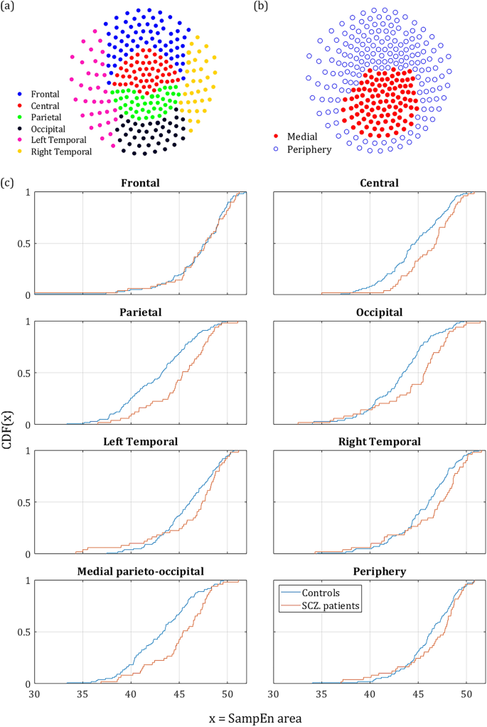
To further study the anatomical characteristics of the MSE values, we calculated the difference in κ between controls and SCZ patients for 6 different scalp areas: Frontal, Central, Parietal, Occipital and Left & Right temporal lobes (Fig. 2a). The values of κ were calculated across the full range (4–80 SF). The largest difference was found in the parietal and occipital areas (Fig. 2c). The central area also showed a substantial difference between the groups. The temporal lobes showed a moderate effect and there was practically no effect in the frontal lobe. The results of all SF ROIs and scalp areas are summarized in Table 1 and Fig. 3. To test the robustness of the effect to differences between SCZ and Controls, and to exclude possible biases, we tested the same effect across sex and handedness. The test across sex reached significance in 46 out 273 channels. This result could be expected, since the groups were unbalanced in that respect (67% and 37% males in the SCZ and control groups, respectively). The test for handedness yielded no significant channels at all (See supplementary Information).
Differences in MSE across different anatomical areas. (a) anatomical areas according to conventional EEG/MEG mapping60. (b) suggested mapping according to our results, dividing the scalp into medial parieto-occipital region and periphery. (c) The CDF of κ averaged across different anatomical locations along the scalp. It is noticeable that Parietal Occipital and Central lobes exhibit a more pronounced difference than the frontal and temporal sensors. However, the largest difference was found in the middle of the scalp.
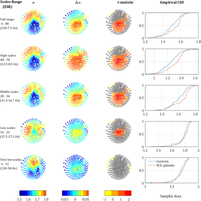
SampEn strength for different scale ranges. The left column depicts the sensors mapping of the κ value averaged across both populations (each dot represents a sensor). The second column depicts Δκ, the difference between SCZ and controls. The third column presents the t-statistic value of sensors which reached significance of p-value below 0.05 (t-test, uncorrected). The rightmost column depicts the CDF curves of the κ values in SCZ and controls. Each row represents a different range of scales. Full range (Broadband), high, intermediate, low, and very-low. In brackets is the equivalent sampling rate (ESR).
Out of the sensors that reached significance, in 120 the κ value was higher for the SCZ patient and only 4 sensors showed a higher κ for controls. All 4 were located next to each other at the left edge of the frontal cortex between the frontal and left temporal areas (yellow dots in the t-statistic column of the upper row in Fig. 3). The rest of the significant sensors were located mostly in the occipital-parietal cortex with few sensors at the edges of the right and left temporal areas. More careful examination reveals that out of 124 sensors with significant difference in Δκ, 113 sensors were located around the posterior frontal, parietal, and the anterior occipital lobes. Therefore, we suggest dividing the scalp into two regions (Fig. 2b): the medial parieto-occipital region, which shows low SampEn κ (high complexity) and high Δκ, and the periphery, in which the SampEn is higher and the difference between groups, Δκ, is much lower.
The upper row in Fig. 3 depicts the κ and Δκ across all scales and the corresponding.
t-statistic for each sensor. It is quite noticeable, that the low κ values (hence low entropy or high temporal correlations) are concentrated at the back-middle of the scalp (mostly central parietal and occipital). Moreover, the difference between the SCZ patients and controls Δκ also peaks at the center of the scalp and correlates strongly to low κ. This can be expected because the areas exhibiting lower entropy (or high temporal correlations) are the areas where one would expect to find a higher difference. The Cumulative Distribution Function (CDF) curves of the κ values for controls and SCZ patients is shown in the rightmost column of Fig. 3.
Scale range analysis
We further analyzed the behavior of the SampEn vs. range of SF. We extracted κ for the regions around the 3 peaks that were observed along the difference (ΔSampEn) curve (Fig. 1c,d) and added to it another range of Very Low Scales (VLS), hence high frequencies. The ranges are summarized in Table 1 and the results of the analysis after breaking down to different ranges are depicted in Fig. 3. The analysis shows a clear trend, according to which not only the difference Δκ between SCZ and controls increases with scale, but also the significance as expressed by t-statistics (middle column) and the difference between the Cumulative Distribution Function (CDF) curves of the κ values (left column). These results are in good agreement with recent work, which stresses the abnormality found in the α and δ power bands in SCZ patients3.
Phase-shuffling analysis
To tease apart the contribution of the amplitude component (or the linear component) to the entropy from the contribution of the phase component (the nonlinear component), we generated a phase-shuffled signal from the original time series for each participant and applied the same MSE analysis to it (see methods).
As expected, the phase-shuffled signal (PSF) yielded a significantly higher SampEn in all.
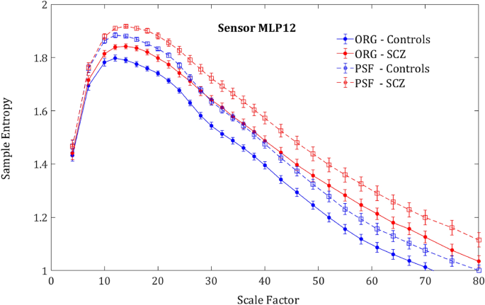
participants in comparison to the original signal (ORG), indicating a decrease of the order due to loss of long-range temporal correlations (Fig. 4). One could expect that the entropy difference between the groups would diminish due to more substantial order decrease in controls, who had more order in the original signal. However, rather surprisingly, the entropy increment obtained by phase-shuffling was slightly larger for SCZ patients (Figs. 5 and 6) and actually increased the difference between the SCZ patients and controls in contrast with the naïve expectation. This outcome was consistent across all channels and scales.
Phase shuffled MSE. SampEn grand averages across groups of MLP12 sensor. Solid lines represent the SampEn of the original signal and the dashed lines the SampEn of the phase shuffled signal. For both groups, the shuffled signal produced noticeably higher SampEn values due to loss of order originating from phase correlations.
MSE differences by component. The upper row shows the SampEn grand average across all sensors and subjects, for the original signal (left column), Phase shuffled signal (middle column) and the difference between the two (right column) i.e., the phase component. The middle row shows the difference in SampEn between the two curves of the upper plot correspondingly. The lower row shows the same difference plotted against the corresponding frequency (ESR). The colored areas correspond to the regions in Fig. 1 and the values are specified in Table 1.
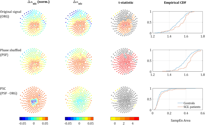
Phase-shuffled MSE across channels. The left column depicts the normalized Δκnlc between SCZ and controls, each dot represents a sensor. The second column presents the absolute Δκnlc, and the third column presents the t-statisic value for sensors that reached significance (p < 0.05, uncorrected). The rightmost column depicts the cumulative distribution function (CDF) of κ values averaged in SCZ and controls. The upper row represents the results derived from the analysis of the original signal, the middle row represents the analysis of the phase shuffled signal, and the lower row represents the NLC. The color scale is equal for all 3 Δκ (Original, PSF and NLC) in both the first and second columns.
SampEn extracted from the PSF time series yielded more substantial difference in term of κ values than the SampEn extracted from the ORG time series, as can be seen in the CDF curves in the right column in Fig. 6 (note the area enclosed by the two curves). Substantial differences were also found in terms of Δκ as shown in the left column of Fig. 6 and the 2nd row in Fig. 5, and t-statistic as demonstrated by in the 3rd column of Fig. 6.
The κ value of the Phase Component (PSC) is defined as the difference between the κ values of the PSF time series and the original time series, \({\kappa }_{\text{nlc}}= {\kappa }_{\text{psf}}-{\kappa }_{\text{org}}\). For most of the sensors, the difference in κnlc between the groups was not significant (lowest row in Fig. 6). However, when averaging across all sensors and all subjects, this difference was significant. Moreover, it did show a clear trend both across scales and sensors, as can be seen in the right column of Fig. 5 and the low row in Fig. 6. These results indicate that the difference between SCZ patients and controls associated with the order generated by LRTCs might be more substantial than a naïve analysis would predict.
Analysis of the phase component
It is noticeable that mean Δκnlc between the groups is much larger than Δκpsf and Δκorg (second and third rows in Fig. 5; note the difference in the scales of the y-axes). This phenomenon is also demonstrated by the sensor mapping (Fig. 6). The sensor mapping also reveals another unpredicted phenomenon, namely the clear spatial trend of the NLC. While the Δκnlc values in the central ROI are fluctuating around zero, in the periphery Δκnlc is clearly positive. Yet, Δκnlc has reached significance only on 10 sensors in the peripheral ROI, due to the small amplitude of the κnlc (rightmost column in Fig. 6) relative to \({\kappa }_{\text{psf}} \text{and} {\kappa }_{\text{org}}\) and fluctuations in their values. To see whether this phenomenon is substantial, we depicted (2nd column in Fig. 6) the mapping of Δκnlc and Δκ’nlc. The mapping of Δκnlc reveals that the magnitudes of Δκpsf and Δκnlc have contradicting spatial trends and, actually, look complementary to each other. To test whether this phenomenon is significant, a t-test was performed between the values of R ‘and ΔR of SCZ patients and controls. The difference in both values was found to be significant with p < 0.05 for R’ and p < 0.013 for ΔR.
Classification using MSE features
To test the potential of MSE as a biomarker, we designed a classification test to compare the classification potential of MSE features versus conventional features extracted from the Power Spectral Density (PSD). We also compared it to LDA classification performed with 6 features extracted from performance in the n-back paradigm.
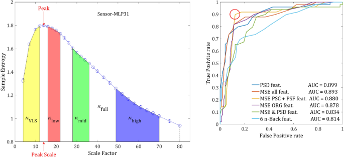
First, we extracted from the MSE scores of the original time series (ORG) for each channel of each participant the following features (Fig. 7): 5 κ values derived from 5 scale regions full, high, mid, low, and VLS (see Table 1), peak value (the highest SampEn value for a given channel) and peak-scale (which is the scale in which the peak was found). The features were then averaged across channels for each of the 2 ROIs: central and periphery, as was previously suggested according to the anatomical analysis, (Fig. 2b) to produce 14 features from the original time series. For each of these 14 features 4 values were calculated across each sensor ROI: mean, maximum, minimum and the Standard Deviation (SD) for a total set of 56 (\(14\times 4\)) MSE features for each participant. The same set of 56 features were extracted from the Phase Shuffled Time Series for (PSF) and from the time series of the Non-Linear Component (NLC) for a total of possible 168 features.
classification. (a) features extracted from a single channel. The 7 features that were extracted from each channel: κ values of the VLS range (yellow area), low range (red), mid-range (green), high range (blue) and full range (denoted by the dashed line). The peak is the highest SampEn of each channel and the peak-scale is the scale at which the peak value is found. (b) ROC curves ROC yielded by the LDA classification procedure applied on MSE features set (in blue), PSD set (orange), N- back set (purple) and MSE & PSD merged set (yellow). The red circle indicates an optimal threshold of the merged features set allowing a sensitivity of 0.857 with specificity of 0.215.
To study the classification potential of different feature sets, and to find which features are the most discriminative, we designed a training and validation procedure, based on simple LDA classifiers and utilizing the multi-realization approach (see supplementary Information). To set the chance level of the validation group to 50%, it was truncated to match the number of SCZ patients and controls. For instance, if the validation group had 17 patients and 27 controls then 17 random controls were drawn to match the number of patients.
At first, to get an idea for the minimal number of features needed to reach the best accuracy, we added lasso regularization to the LDA classification procedure and scanned the regularization hyperparameter λ between 0.02 and 0.4. The number of significant features dropped rapidly to 8 features at λ = 0.12, then to 3 features (λ = 0.28) and finally converged to 2 features at λ = 0.37. However, the accuracy for 2 or 3 features was considerably lower (73% ± 5%), than for 10 features (78.5% ± 5%). Further increasing the number of features did not have any significant effect on the accuracy.
Next, we applied the classification procedure to each of set of features (ORG, PSF & NLC) separately and then to combination of 2 sets and finally all the 3 sets together. The ORG and PSF features yielded very similar results (~ 77%). However, the PSF set converged faster, perhaps as a result of the slightly larger magnitude of PSF features. Although the NLC set alone yielded the poorest results, when combining it with ORG or PSF sets the accuracy increased by 3–4%. This result strengthens the findings that the NLC component contains additional information. The combination of PSF & NLC and ORG & NLC yielded very close results, which could be expected since the magnitudes of ORG and PSF features are of the same order and about 10 folds larger than the magnitude of NLC. There is practically no increase when combining all 3 sets together. In terms of Receiver Operating Characteristic (ROC), all the feature sets except for the NLC yielded an AUC (Area Under the Curve) between 0.8 and 0.9 (Table 2 & Fig. 7). The joint of all 3 feature sets yielded the slightly highest AUC of 0.899. However, the set of PSF & NLC yielded the most balanced ROC curve (Fig. 7), allowing a considerably better optimal threshold. The sensitivity and specificity were 0.898 and 0.122, respectively. The results are summarized in Table 2.
When trying to select a minimal subset of the most discriminative features, we noticed a considerable multi-collinearity among different features and particularly between the mean and max values of the same features. After resolving most of the collinearity issues (see supplementary Information) we converged to a subset of 14 features, each of them is allowed to interchange between the mean and max values. The accuracy of the minimized subset came close to the original set yielding 76.2 ± 6% and AUC = 0.828 (Table 2).
Comparison with power spectrum density based classification
To examine whether the MSE analysis has an advantage over conventional power spectrum features (in terms of classification power), we applied a similar LDA classification procedure to compare the discriminative power of MSE derived features to PSD features. From each channel we extracted the conventional power bands δ, θ, α, β, γ and averaged their magnitude across the 6 conventional ROIs in EEG/MEG analysis: Frontal, central, parietal, occipital, left and right temporal (Fig. 2a). We also added the 2 ROIs used in the MSE analysis (Fig. 2b) and the total ROI (all the sensors), for a total of 9 ROIs and accordingly 45 features (5 bands \(\times\) 9 ROIs). For each of these 45 features, 4 values were calculated across each sensor ROI: mean, max, min and the standard deviation for a total of 180 values representing the power spectrum of each participant. Next, we performed the same classification procedure as for MSE features. The results were similar to MSE and converged to accuracy of 77.8 ± 5.3% and AUC = 0.834. The most discriminative features were related to δ and α power bands in agreement with the existing literature3. Lastly, we tried to merge the features of MSE and PSD to see whether the joint discriminative power would increase. The best 20 MSE features were added to the best 20 PSD features to form a joint one set of 40 features. The same LDA classification procedure was applied to the joint set. Both accuracy (79.7 ± 5.4%) and AUC (0.876) slightly improved converging to almost the same values as MSE features alone.
Comparison with a cognitive task (n-back)
The results of each n-back block are given by two variables: accuracy and reaction time (RT). Since each participant was asked to perform 3 blocks (n = 0, 1 & 2), this results in 6 variables representing each participant’s performance: Score0, Score1, Score2, RT0, RT1 & RT2 for n = 0, 1 & 2, respectively. After discarding participants who did not perform or did not complete the task as required, we were left with 129 participants in total (42 SCZ patients and 87 controls). Performing the same classification procedure as for MSE and PSD features yielded very similar results (Table 2). When comparing the discrimination of a single feature, the n-back feature gives a slightly but not significantly better result. When comparing three n-back features, the results were equivalent to that of 10–15 MSE or PSD features. The most discriminative feature was Score2, followed by RT2 or Score1, the remaining 3 did not contribute much to classification.
XG boost classification
To make sure we thoroughly explored the discriminative power of the MSE method, we applied a different method of classification, the XG boost method that is based on a decision tree. We applied it to the representative subset of the 28 features. The results were quite similar, with accuracy around 76% independent of the initial parameters, and the best AUC was 0.791.

