Participants
All participants were clinically stable adult outpatients with schizophrenia spectrum disorder (SSD) (Table 1) and provided written informed consent; all study protocols were approved by relevant review boards.
Dataset I (N = 282) was used for both Objectives I & II. Participants were drawn from the multi-site social processes initiative in the neurobiology of schizophrenia(s) (SPINS)28 and underwent the full range of assessments below. Recruitment took place at the Zucker Hillside Hospital (Glen Oaks, NY), the Centre for Addiction and Mental Health (Toronto, Ont.), and the Maryland Psychiatric Research Center (Baltimore, MD). The assessments were conducted across three visits (MRI, neurocognition, social cognition, clinical assessments, and participant self-reports). For these analyses, we selected SSD participants who had completed assessments for functioning. SSD participants met the Diagnostic and Statistical Manual of Mental Disorders, 5th Edition (DSM-5) criteria for schizophrenia, schizoaffective disorder, schizophreniform disorder, or unspecified psychotic disorder. Other aspects of this cohort, along with further details about the recruitment, ascertainment, and assessments, have been previously described by Oliver et al.28, Hawco et al.29, and Tang et al.30.
Dataset II (N = 317) was a validation set for Objective I and underwent functional outcomes assessments. Imaging and social cognitive phenotyping were not available, so this Dataset was not included in Objective II. Participants were recruited primarily from the Zucker Hillside Hospital, with adjunctive recruitment conducted at the Manhattan Psychiatric Center. For these analyses, we selected SSD participants who had complete functional outcomes assessments, and who did not re-enroll in the SPINS study. SSD participants met DSM-IV-TR criteria for either schizophrenia or schizoaffective disorder. An interim analysis from this dataset, along with further details about the ascertainment and assessments, have been described by Shamsi et al.31.
Assessment of functioning
For Dataset I, functioning was assessed with the Birchwood social functioning scale (BSFS)3 and quality of life scale (QoL)5, both clinician-rated scales based on participant reports. Each subscale was considered separately.
For Dataset II, related functioning domains were assessed, though with different scales and modalities. We used the following items: work and interests from the Hamilton rating scale for depression (Ham-D; clinician-rated)32, role and residential functioning from the multidimensional scale of independent functioning (MSIF; clinician-rated)4, leisure activities, social frequency, and degree of social activity from social adjustment scale (SAS; self-report)33, and financial and communication skills from performance-based skills assessment (UPSA; performance-based)4. Table 2 and the Supplemental Methods include further details.
Assessment of biopsychosocial measures
Biopsychosocial measures were evaluated as correlates of functional phenotype for Objective II (Dataset I). Detailed descriptions are listed in Supplemental Methods and Table 3.
Sociodemographic and personal characteristics
We used participant report and electronic health records (EHR) to determine self-identified demographic information and personal characteristics potentially relevant for functional outcomes, including family history of SSD, English as primary language, parental educational attainment (highest known), and duration of illness for SSD.
Assessment of Biopsychosocial MeasuresClinical Symptoms
Psychosis symptoms were assessed using the Brief Psychiatric Rating Scale (BPRS)34 and the Scale for Assessment of Negative Symptoms (SANS)35. Subscale scores were used to represent different symptom domains.
General neurocognition
General neurocognition was assessed with the NIMH-measurement and treatment research to improve cognition in schizophrenia (MATRICS) consensus battery36. (The Mayer–Salovey–Caruso emotional intelligence test (MSCEIT) was categorized with the social cognition measures)37. T-scores for each domain, i.e., processing speed, attention and vigilance, working memory, verbal learning, visual learning, and reasoning/problem-solving, were used.
Social cognition
Emotional intelligence, emotion processing, mental state attribution, and social perception were assessed with: the MSCEIT; the Penn emotion recognition 40 (ER40)38; the awareness of social inference test-revised (TASIT)39; the reading the mind in the eyes task (RMET)40; and relationship across domains (RAD)41. The assessments were chosen to cover a range of social cognitive domains because of their inclusion in the social cognition psychometric evaluation (SCOPE)42.
Subjective psychological experiences
Self-report questionnaires assessed subjective experiences of interpersonal situations with the interpersonal reactivity index (IRI)43 and the schizotypal personality questionnaire-brief version (SPQ-B)44.
MRI
Brain volume measures representing replicable structural MRI findings in schizophrenia45 were included as potential predictors (Table 3). The rationale was that key biological signals associated with SSD diagnosis may converge on the level of brain structure, and may be associated with functional phenotypes in SSD. That is, individuals with higher biological loading for schizophrenia may show more pronounced differences in brain structure as well as greater functional impairment. Magnetic Resonance Imaging (MRI) was performed on six 3 T scanners across the 3 sites and harmonized as previously described by Oliver et al.46,47. Imaging parameters and additional details can be found in the Supplemental Methods. T1-weighted anatomical images were corrected for intensity non-uniformity (INU) with N4BiasFieldCorrection48, distributed with ANTs 2.2.0 (RRID:SCR_00475749). Brain surfaces were reconstructed and subcortical volumes were calculated using Freesurfer recon-all (FreeSurfer 6.0.1, RRID:SCR_00184750). The selected volumetric measures (Table 3) represent replicable structural MRI findings in schizophrenia Right and left hemisphere measures were included separately.
Objective I: defining functional phenotypes
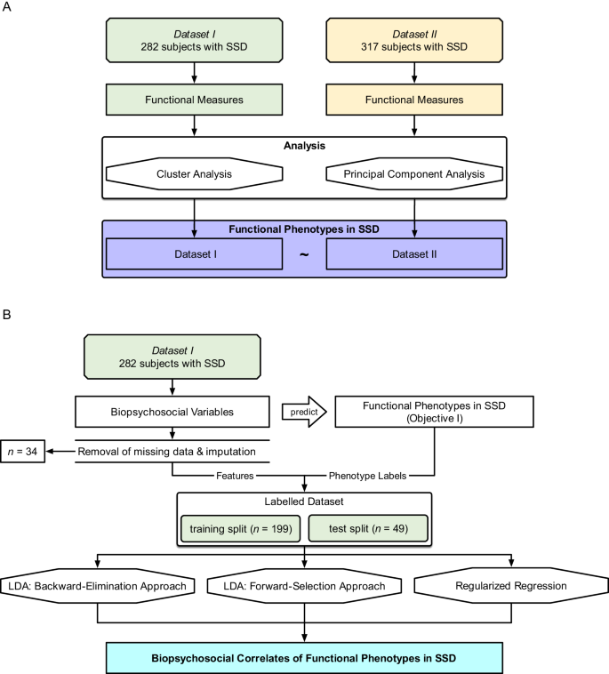
Objective I was tested on both datasets, with Dataset II as an independent validation sample (R packages listed in Supplemental Table 1). The aim was to define functional phenotypes based on patterns in the expression of individual functioning measures (Table 2) using an unsupervised clustering approach with bootstrapping. This approach was chosen because, assuming that the samples are representative of the larger SSD population, clustering informs us about the functional phenotype patterns which we might expect to observe among patients in a clinical setting. Additionally, a principal component analysis was performed to describe functioning domains and aid interpretations of the functional phenotypes. The analysis pipeline is shown in Fig. 1A.
A Objective I: Defining functional phenotypes. Two datasets (\({N}_{I}=282\), \({N}_{{II}}=317\)) were analyzed separately, and unsupervised clustering and principal component analysis were performed on individual functioning items to define 3 functioning phenotypes. B Objective II: Predicting functioning phenotypes (Objective I) based on demographics, neurocognition, social cognition, and brain structure. Thirty-four participants were excluded from Dataset I due to insufficient data; resulting in \(n=248\) remaining participants. We performed three methods (backward-elimination LDA, forward-selection LDA, and regularized regression).
Cluster analysis
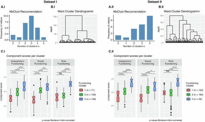
We performed bootstrapped hierarchical Ward clustering across the individual functional items51, optimizing Euclidean distance. The optimal number of clusters (n = 3) was determined using the NbClust R package in Dataset I based on 11 functioning items (Fig. 2). For Dataset II, clustering was conducted on 8 functioning items. From NbClust, 11 of the metrics proposed \(k=5\) clusters as the optimal cluster number; the runner-up was \(k=3\) with 7 indices suggesting this as the optimal cluster number. For consistency, 3 cluster solutions were produced for both datasets. Bootstrapping was performed 100 times in each sample using the clusterboot function from the fpc R package to determine optimal clustering and cluster stability. To compare functioning and biopsychosocial variables among the three clusters, we used pairwise t-tests with Bonferroni–Holm-corrected p-values52. Group effects for demographic variables were evaluated using ANOVA for age and clinical ratings and Fisher’s Exact test for sex, race, and diagnosis. The generalizability and stability of the clusters were established by running the analyses on independent samples, using different functioning items; resampling was not employed.
Subplots A.I and A.II depict the frequency of NbClust provided indices that recommended a certain cluster size for each dataset. Subplots B.I and B.II show the hierarchical clusters produced by the Ward algorithm (applying a Euclidean distance as a distance metric). Subplots C.I and C.II compare the functional phenotype clusters based on the functional components resulting from the PCA. Higher component scores reflect better functioning in that domain. Pairwise comparisons (\(t\)-tests) were used to evaluate statistical significance (Bonferroni–Holm-corrected52: ns not significant, *p < 0.05, **p < 0.01, ***p < 0.001, ****p < 0.0001).
Principal component analysis
To aid interpretability, principal component analysis (PCA)53 was performed on the individual functioning measures. The scree plot was visually inspected, and Kaiser’s criterion was used to determine the optimal number of components (Supplemental Fig. 1). For both datasets, we used a three-component solution with Promax rotation.
Objective II: Identifying Biopsychosocial Correlates
Objective II was tested on Dataset I. The aim was to identify the subset of biopsychosocial correlates which, when taken together, most accurately classify participants into the 3 functional phenotypes defined in Objective I. We evaluated 65 intercorrelated biopsychosocial variables including sociodemographic and personal characteristics, psychosis symptom ratings, general neurocognition, social cognition, and structural brain imaging metrics (Table 3). The emphasis was on understanding how different combinations of biopsychosocial correlates may be related to functioning, and not on building a classification model per se. The analysis pipeline is shown in Fig. 1B. Variables which may not have a main effect on functional phenotype were nevertheless included because of the possibility of secondary interactions with other variables.
Preprocessing
Due to missing values in biopsychosocial measurements, we implemented an exclusion-imputation strategy. We removed 34 individuals from Dataset I who had 4 or more measures missing (5% of the total feature set). For individuals with 1–3 missing measures (\(n\) = 28), we imputed these using the mice R package and predictive mean matching, resulting in a total sample size of 248 individuals from Dataset I. A total of 40 observations were imputed out of over 16,000 (0.2%). After imputation, an 80/20 train-test split was made. In order to normalize coefficients and avoid bias from the test set, each of the 65 predictors was standardized by calculating z-scores with respect to the training split. Sample characteristics for both the train and test set are shown in Supplemental Table 2.
Latent discriminant analysis (LDA) classification
We selected linear discriminant analysis (LDA) as our classification algorithm due to a) its ability to perform multi-class classification suitable for the 3 functional phenotypes and b) its interpretability and ability to provide variable coefficients (i.e., linear discriminants; LD) that determine the strength and directionality (i.e., positive or negative) of the contributing predictor. Two LDs were examined because LDAs are limited to a dimensional space lower than the number of groups being classified (3 clusters—1 = 2 LDs). The LDA function from the MASS R package was used. The training was done on an 80% training set using leave-one-out cross-validation. The generalizability of the resulting model was determined on a 20% set-aside test set. The whole dataset was used for reporting the final LD coefficients. The target metric for the classification was accuracy: i.e., the percentage of correct classifications.
Backward-elimination linear discriminant analysis
The aim was to identify an interpretable set of key correlates out of the 65 biopsychosocial predictors (Table 3) that best describe the functional phenotype. A limit of up to 10 variables was defined a priori. Ideally, we would evaluate all possible combinations of variables at each level from 1 to 10 (e.g., level 4 would test all combinations of k = 4 variables out of the n = 65 possible predictors). However, trying every combination of \(k=10\) variables for \(n=65\) total predictors would result in almost 180 billion combinations (see Supplemental Table 3). A feasible computational boundary was, therefore, set at 2 million variable combinations. To keep the number of combinations below this threshold at each iteration, we applied a stepwise elimination (i.e., backwards elimination) of predictors that contributed least to the prediction performance in the previous step, i.e., lowest average test-set accuracy.
The variable selection proceeded as follows: if the number of combinations in a given level exceeded the computational threshold, we eliminated poor predictors until the threshold was met. Poor predictors were defined as the predictors with the lowest maximum accuracy in the previous level. An overview of the eliminated variables and combination counts is provided in Supplemental Table 4. For example, at level 5, 16 variables were eliminated in order to stay within the computational threshold; so, we selected all k = 5 combinations from n = 49 variables and ran a total of 1,906,884 LDA models. This was continued until we reached level 10 consisting of 10 predictors.
Forward-selection linear discriminant analysis
With the aim of identifying an interpretable set of key correlates without a pre-defined limit to the total number, we developed an approach using a successive forward selection of predictors and a natural, data-driven stopping point. For each iteration, the best combinations of one, two, three, and four variables were identified—due to these being within our computational boundary of 2 million (Supplemental Table 3). A predictor was selected (i.e., “fixed”) if it appeared in at least 3 of 4 best performing models (based on test-set accuracy), allowing for interaction effects where a predictor may be valuable in combination with other predictors, but not on its own. Selected predictors were added iteratively to the fixed predictor set and included in all subsequent levels. This process terminated when no further consistent variables were found.
More specifically, for the first iteration, we evaluate all 1–4-variable combinations of the 65 predictor variables from Table 3. Two predictors appeared in 3 or more of the best-performing models (Avolition and Anhedonia). These were then fixed as predictors, and included in all subsequent iterations. For the second iteration, we tested Avolition and Anhedonia in combination with all 1–4-variable combinations of the remaining 63 predictor variables. This time, Left Hippocampal Volume was selected as a fixed predictor. For the third iteration, we tested Avolition, Anhedonia, and Left Hippocampal Volume in combination with all 1–4 variable combinations of the remaining 62 predictor variables, and so forth. Variables were added over 4 iterations. For the fifth iteration, none of the remaining variables appeared in 3 or more of the best-performing models, so the process reached its natural termination.
Regularized regression
To validate the findings from the LDAs, we used the L1 regularized regression, i.e., least absolute shrinkage and selection operator (LASSO) using the R glmnet package as a penalizing regression that performs variable selection and prediction in one step54. However, this regression functions as a binary classification and cannot be directly applied to a three-class problem. Thus, we applied a one-vs-rest strategy—computing two models that were analogous to the two latent discriminants from the LDAs described above. The appropriate model \(\lambda\) hyperparameter was determined using the minimum mean cross-validation error. We report the archived accuracies on the training and test sets, as well as coefficients for the non-penalized predictors. These coefficients were determined using an L2-regularized regression, i.e., ridge regression, trained on the entire dataset using the L1-selected predictors to allow for the retainment of the selected predictors.
Of note, the regression was used primarily to validate findings from the LDAs, and is limited by its inability to classify all three clusters in the same model. The 2-class prediction accuracies reported for the LASSO one-vs-rest should be interpreted on a difference scale from the 3-class prediction accuracies performed with the LDA because the random-guessing accuracy is 50% for a balanced two-class prediction problem, and 33% for a 3-class prediction.
Constructing a final model
Predictors emerging consistently from both the backward-elimination and forward-selection LDAs (the primary methods) were identified as replicable key correlates of functional phenotype. The key correlates were used as predictors for a final LDA model describing the full sample to provide a unified summary of the LDA results. We recorded the confusion matrix of the final model as well as accuracy and balanced accuracy—defined as the average of the recall of each of the three classes.


